Pushing Aside the Bench for the Mark: Choosing an LLM For Your Product

Benchmarks Are General

When you go to any of the popular benchmark leaderboards, it is like looking at a list of “here are the fastest and most capable athletes.” But a general athlete is not what you need; your use case needs a swimmer. They must be capable, but in what exactly: technique, resilience under pressure, or something else? They need to be fast too, but in 100m backstroke or getting to the pool? It turns out your use case is for an open water swimmer capable of swimming the English Channel.

This is the essence of why you cannot simply make your choice by popular benchmarks. They rank in general, but your use case is never general.

Below I will setup a fictitious (and overly simple) example of needing to choose between the five Anthropic models. The purpose is to help you establish a fundamental way of thinking about model selection.

Choosing An Anthropic Model

Assume that for my fictious use case I need to decide between the following five Anthropic models:

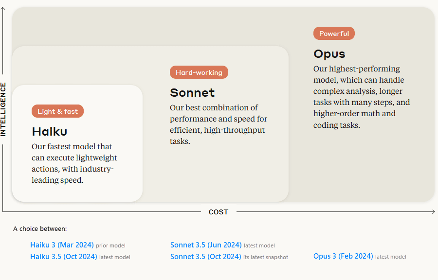
Looking at the above Sonnet 3.5 seems to be the easiest choice, and I assume the (Oct 2024) snapshot must be even better. The leaderboards point to this too, but is it?

It depends entirely on your use case. The way to test this is by evaluating or “marking” prompt responses. Not just generic prompts but a set of prompts with representative coverage of your use case. The more coverage you have and the more relevant the prompts, the more confident you will be in choosing a model (or validating a move to the latest version/snapshot).

For this article, I will make evaluating my use case (unrealistically) simple by “marking” model responses on just two prompts:

Speed Test (prompt 1)
Explain photosynthesis in a concise paragraph. (max_tokens: 400)

Capability Test (prompt 2)
What is the geometric monthly fecal coliform mean of a distribution system with the following FC counts: 24, 15, 7, 16, 31 and 23? The result will be inputted into a NPDES DMR, therefore, round to the nearest whole number.

As LLMs deal in probabilities, the same prompt can have different responses. Model speed can fluctuate too. To address this, I chose to run each prompt 50 times against each model (5 x 2 x 50 = 500 total runs). While 30 (not 50) runs is typically sufficient for statistical significance, I opted for 50 runs as I was unsure of variability.

The results below were gathered from a full test run done on the 4^th of February 2025 at 15:02 UTC. The 500 prompts and their responses finished 16 minutes later.

Now for a step through the results (and surprises) for speed, capability, and cost.

Speed Test Results

Like measuring typing speed in words per minute, model speed is measured in tokens per second. This measures the total time from sending your prompt request until receiving the response – including both the model’s “thinking” time (inference) and the internet journey time. This is the speed your product will experience. See Appendix II for the code snippet used.

Looking at Figure 1 (above), perhaps you are assuming the same as I did. That the Haiku models will be fastest, and that Haiku 3.5 will be faster than Haiku 3.0. As the results will show below, both assumptions turned out to be wrong.

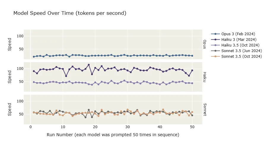
Figure 2 above shows “speed over time” for the speed test prompt that was sent 50 times to each model, in sequence. The are clear differences in speed despite the fluctuation between runs. Looking at the same in a more comparable format:

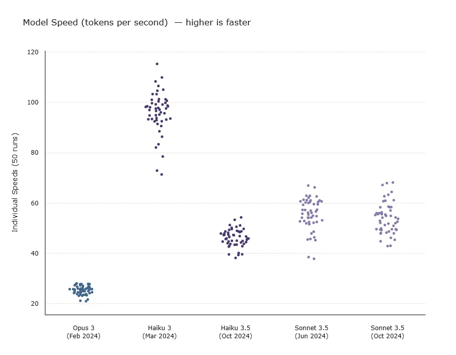
What is most surprising is that the newer Haiku 3.5 appears to be slower than Sonnet 3.5 (both snapshots). Also, although Opus is an order of magnitude slower its speed is much more stable (notice the differences in vertical spread).

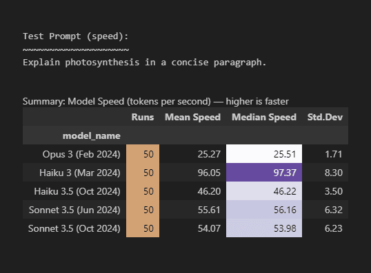
Figure 4 above is a full summary of the speed test results. I chose the median to compare speed because of outliers and being slightly skewed (mean ≠ median). If this were the real world and speed crucial, ensure observed speed differences are statistically significant.

If we were choosing for your swimmer use case, so far Haiku looks the best although its performance is least dependable (look at the spread of the dots in Figure 3 and the standard deviation in Figure 4). And of course, this is only speed, is it capable of swimming the English Channel?

Capability Test Results

Capability is easy to measure when a definitive response is expected, like a math solution or classification. Typically, you will need to compare textual responses. In this case, there are several methods, both manual and automated, that can be used to evaluate or “mark” textual responses for comparison. In my opinion, the most promising is using an independent LLM to judge the responses; it can be automated and is more consistent than within and between people¹.

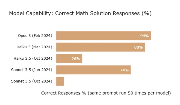
The capability test prompt used (Figure 5 below) has an exact solution of “18”. You can see that even for Opus, “the most intelligent model,” is not infallible and got 6% of its answers wrong:

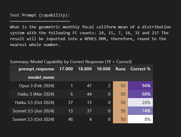
Like speed, the results for my “use case” contradict the benchmarks. Sonnet should be outperforming Haiku. And like with speed, both Haiku 3.5 and Sonnet 3.5 (Jun 2024) degraded from their predecessors. What does hold true is that Opus did top as most capable, although surprisingly it is Haiku 3 and not Sonnet 3.5 that comes in as close second.

You can easily imagine that speed tests are affected by the day of the week you run the test on and where you are getting your model served from (e.g., AWS or Anthropic themselves). But if you think you are in clear with capability, I can tell you absolutely no. Please see Appendix II. I may have just caught a rare event, but unexplained variation happened to me with this example.

It is now time to look at what appears at first glance to be the easiest of all: comparing costs.

Cost Calculations

I used to work in manufacturing where products were sold to mines, shipping companies, etc. Buyers unconnected to ground operations would opt for cheaper suppliers. The cheaper products would fail sooner or require more maintenance. The client would suffer far more costly repercussions, but of course invisible in quarterly budgets. Nobody can blame the buyers — everyone likes the look of a low price.

In the LLM world, most providers price models in “cost per token”. However, it is more complex than a simple comparison as a token is not standardised. For example, Anthropic may tokenise a given sentence as “12 anthropic tokens”, whereas Open AI may tokenize it as “14 open ai tokens”.

The trick is to first delve into deeper cost questions before considering quoted prices. For example, do you get accurate responses efficiently or does it require multiple back and forth (more tokens)? For a hosted model, does it get congested and what will this cost your product? Is the API easy and robust to use so your team can move quickly? Is there documentation on prompt engineering practices for the model? Regarding privacy, how much is that going to cost if things go wrong? Once you have considered these deeper costs, only then standardise and compare the easy token costs.

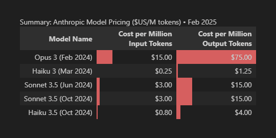
Anthropic prices their models in dollars per million tokens ($/MTOK), with input tokens costing less than output tokens. You can see where this is going: which price is more important to your use case? Is it possible to cache prompts? And if relevant to your use case, how much could you save?

Current³ Anthropic pricing:

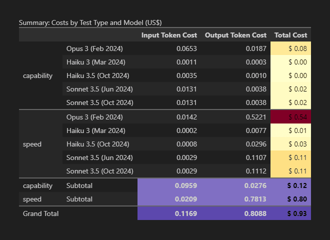
It cost $0.93 to run the entire test set of 500 prompt requests. In the detailed breakdown below, the speed tests cost more because a “concise paragraph” was asked for. Whereas the capability prompt instructed “respond only with a number”.

It is obvious now that while developing your product at scale, prompts can be optimised for cost efficiency. But first, you need to ensure the model is fit for your use case. Then, look at the entire cost picture in place of the seemingly easy-to-compare token costs.

Results Summary

Figure 9 below summarises all the results into one diagram. On the x-axis are the median speed test results (running prompt 1 against each model 50 times). On the y-axis are the capability test results (running prompt 2 against each model 50 times). The size of each circle is the total cost, for both speed and capability tests combined.

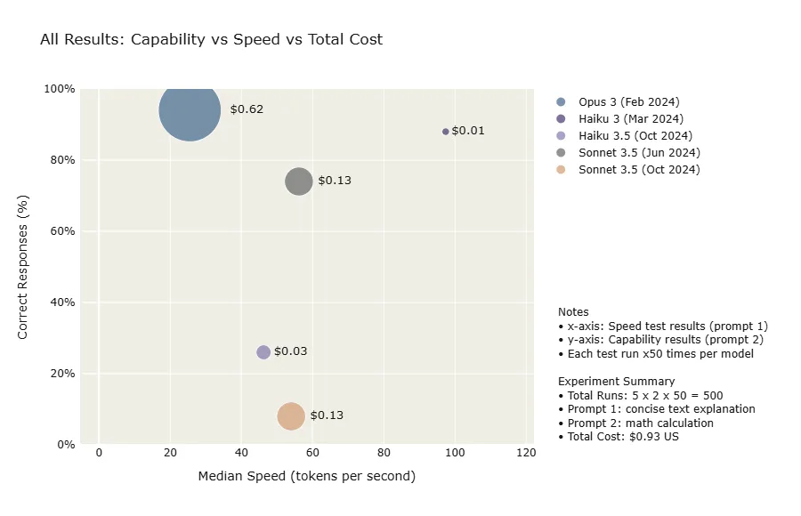
Comparing the benchmarks and Anthropic’s model positioning, when measured against my fictitious use case of just two prompts, here are the biggest contradictions and surprises:

Speed
“Haiku 3.5 our fastest model” — it was not the fastest, Sonnet 3.5 was faster. Both dwarfed by the older Haiku 3. All newer models and snapshots degraded in speed.

Capability
“Sonnet 3.5 our best combination of performance and speed” — it was not, Haiku 3 outperformed Sonnet 3.5 on both. All newer models and snapshots degraded in capability.

Cost — most surprising of all
Haiku 3 is the fastest with the closest capability to Opus — yet it is the cheapest!

Again, though, please keep in mind that two little test prompts are not enough to draw a conclusion, but neither are general benchmarks. What these results prove is that you can expect to find surprises: you need to evaluate against your own use case by testing with use case relevant prompts.

Future Proofing

You certainly will choose the wrong model, if for no other reason that things change rapidly: think of DeepSeek-V3 that arrived in January. If the popular benchmarks are to be believed, it is comparable to Claude 3.5 Sonnet but at $0.28/MTOK⁴ instead of $3.00. That would make your December decision wrong (ceteris paribus).

The perfect choice does not matter nearly as much as your ability to adjust from a “wrong” decision. To do this you must be able to quickly evaluate new models (or updates) against your use case, then to have the built-in flexibility to switch, confidently.

So deeply consider (A) and (B) below:

(A) For evaluating new models:

As your product grows, you add more prompt evaluations for the prompts used by your product. Now not only do you have the evaluations you started off with in choosing your model, but a growing evaluation set truly representative of your use case. Strive for these tests to be automated. With a little work, you can run this evaluation set against other models for comparison.

At DeepSeek-V3 costing roughly 1/11^th of Model 1 (output tokens), it is too difficult to believe that it could possibly be as good. You do not know until you test the model against your own use case. To be able to do this quickly and comprehensively is game-changing.

(B) Making a model switch easier:

From the start, at the very least allow your Engineers to invest in an abstraction layer. Get into a room and explain future proofing, explain the story of DeepSeek-V3 where Sonnet’s cost is 1/11^th of it. Go beyond price – as a team, what will you do when there’s a new breakthrough model that is knocking the lights out on all leaderboards? What will it take to confidently and easily switch? How are we going to easily run our prompt evaluation suite against a new model?

The answer you are likely to get is, at the very least, an abstraction layer that sits between your application’s code and LLM APIs. You do not need a perfect interchangeable model solution, but there are things that, if done with discipline from the start, will keep the product adaptable.

A Zapier Perspective

As a leading automation platform, Zapier has extensively integrated LLMs. In a conversation with me, their VP of Engineering Mojtaba distilled the essence of this article in one breath:

This space (base LLMs) is moving so fast that choosing the “right LLM” is basically the same as “choosing the right LLM for this week”. In other words, the capability to a) quickly evaluate LLMs as they quickly evolve b) quickly adapt/pivot to new models is key (and not so much picking the right one at the moment). This includes ability to evaluate+pivot to LLM based on need. In other words, some LLMs are good at some things and others for another.

Mojtaba Hosseini, VP of Engineering, Zapier.

Conclusion

In the real world, you cannot use only two prompts to compare models; you must strive for good coverage. I think of my product in major segments of LLM tasks. I emphasise more segments than others, but within each, I strive for coverage by creating relevant test prompts that inject real messy data. When it comes to costs, take the time to research the entire cost picture.

Once the model is chosen, the journey has only started. As your product grows and evolves, so too must your prompt evaluation test suite. Today’s decision is likely to be wrong tomorrow.

Benchmarks and marketing are general, your use case is not. Take the time to automate your prompt evaluations. It is an investment that surpasses quarterly budgets. You may need to defend this investment but persist. You are giving the best chance of having your product flourish in a rapidly changing landscape, and to perform well along the way.

And yes, even the product manager must develop a solid understanding of prompting and statistical analysis (beyond just comparing “dots”).

Appendix I: Unexpected Variation

In a previous life as a Six Sigma consultant, one of the first steps was always to check if the data showed patterns related to time. If there are, the sampling plans and analysis had to be adjusted to draw any useful conclusions. This project here was not a rigorous statistical endeavour, but I did run the tests multiple times over 4-7th of February. For capability, I thought I was in the clear as “Correct %” scores looked very similar over these days.

Then by luck I ran my tests again on the 8th of Feb. This day was extraordinary as all the 3.5 models “jumped” in capability, together:

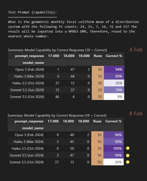
The lesson learnt is to run your tests more than once. Otherwise, you may be unlucky in that you are drawing your conclusions off of a day like my 8th of Feb. I asked Claude.ai to explain the results to me as an “LLM expert”, to guess at what some of the special causes could be of this variation. This is what Claude said:

Potential Technical Explanations:
• Infrastructure Changes
• Backend serving infrastructure might have been modified
• Load balancing configurations could have changed
• Model deployment settings may have been adjusted
• Cache clearing or system updates might have occurred

The Puzzling Aspect:
• The mathematical problem has a single correct answer
• Higher temperature might introduce more variance, but not systematic improvement
• Feb 4-7 showed consistent results

Again: Run your tests more than once to be sure you have not caught an 8th of Feb day.

Appendix II: Code

The code to run and visualise test results is available here; how speed was measured:

from anthropic import Anthropic
import pandas as pd

# Start the timer
start_time = pd.Timestamp.now('UTC')

# Make API request to Claude and wait for response
response = anthrop_client.messages.create(
    model='claude-3-5-sonnet-20241022',
    max_tokens=400,
    messages=[{'role': 'user', 'content': speed_test_prompt}]
)

# Stop the timer
end_time = pd.Timestamp.now('UTC')

# Calculate speed in tokens per second
execution_seconds = (end_time - start_time).total_seconds()
output_tokens = response.usage.output_tokens
tokens_per_second = output_tokens / execution_seconds

Footnotes

1. For a compelling argument of why human evals are not silver bullet, watch Evaluating LLM-based Applications (Databricks) ↩︎
2. Capability tests were run at a default prompt temperature of 1 which explains the unexpected results. On reflection the documentation says: “Use temperature closer to 0.0 for analytical / multiple choice, and closer to 1.0 for creative and generative tasks.” ↩︎
3. See latest Anthropic model pricing here ↩︎
4. See latest DeepSeek-V3 pricing here ↩︎

• LinkedIn